Nutrition
Nutrition Quality is represented by a proxy of the number of portions of fruit and vegetables eaten per week. The following variables from understanding society that measure fruit and vegetable consumption were used:
The equations to generate the nutrition composite are as follows:
Both fruit and vegetable consumption frequency was measured in days per week, and reported as:
Never
1-3 days
4-6 days
Every day
The amount of fruit and veg per day was a continuous variable, indicating the number of portions of fruit or veg eaten on an average day when the respondent eats fruit or veg.
This gives us a continuous nutrition score, composed of the sum of two
proxy values for the amount of fruit and veg eaten per week.
Unfortunately because the days_eating_<>_per_week variables are
ordinal (levels = [Never, 1-3 days, 4-6 days, Everyday]) and not just
the number of days, we can’t calculate an actual value for
amount_per_week.
continuous_density(obs)
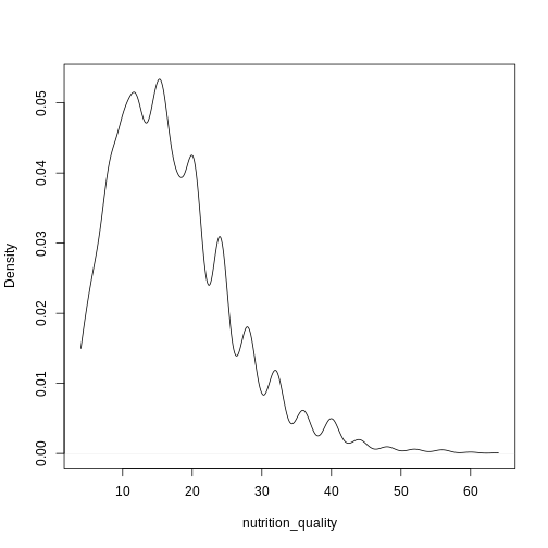
plot of chunk nutrition_quality_data
Transition Model
We use a Linear Mixed Model (LMM) from the lme4 package in R to predict the next state of nutrition quality.
Formula:
print(summary(model))
## Linear mixed model fit by REML ['lmerMod']
## Formula:
## nutrition_quality_new ~ scale(age) + factor(sex) + relevel(factor(ethnicity),
##     ref = "WBI") + factor(region) + relevel(factor(education_state),
##     ref = "1") + scale(hh_income) + factor(behind_on_bills) +
##     factor(financial_situation) + (1 | pidp) + (1 | hidp)
##    Data: data
## Weights: weight
##
## REML criterion at convergence: Inf
##
## Scaled residuals:
##     Min      1Q  Median      3Q     Max
## -3.1107 -0.5698 -0.1088  0.4053 10.4141
##
## Random effects:
##  Groups   Name        Variance Std.Dev.
##  hidp     (Intercept) 2.542    1.594
##  pidp     (Intercept) 2.542    1.594
##  Residual             2.542    1.594
## Number of obs: 70487, groups:  hidp, 49936; pidp, 29227
##
## Fixed effects:
##                                              Estimate Std. Error t value
## (Intercept)                                  16.78024    0.27070  61.987
## scale(age)                                    0.60449    0.03610  16.745
## factor(sex)Male                              -1.39758    0.06502 -21.494
## relevel(factor(ethnicity), ref = "WBI")BAN   -1.73668    0.44716  -3.884
## relevel(factor(ethnicity), ref = "WBI")BLA   -0.67357    0.29203  -2.306
## relevel(factor(ethnicity), ref = "WBI")BLC   -0.93967    0.36796  -2.554
## relevel(factor(ethnicity), ref = "WBI")CHI    0.27003    0.47765   0.565
## relevel(factor(ethnicity), ref = "WBI")IND   -0.91078    0.21522  -4.232
## relevel(factor(ethnicity), ref = "WBI")MIX   -0.18856    0.27254  -0.692
## relevel(factor(ethnicity), ref = "WBI")OAS    0.68035    0.31114   2.187
## relevel(factor(ethnicity), ref = "WBI")OBL    0.82279    0.96326   0.854
## relevel(factor(ethnicity), ref = "WBI")OTH    0.25520    0.50079   0.510
## relevel(factor(ethnicity), ref = "WBI")PAK   -2.17454    0.26700  -8.144
## relevel(factor(ethnicity), ref = "WBI")WHO    1.57690    0.16128   9.777
## factor(region)East of England                 0.01103    0.15545   0.071
## factor(region)London                          0.05260    0.15829   0.332
## factor(region)North East                     -0.21626    0.19899  -1.087
## factor(region)North West                     -0.48531    0.15445  -3.142
## factor(region)Northern Ireland               -1.82362    0.23166  -7.872
## factor(region)Scotland                       -0.73583    0.17327  -4.247
## factor(region)South East                      0.25464    0.14566   1.748
## factor(region)South West                      0.44307    0.15918   2.783
## factor(region)Wales                           0.72114    0.20801   3.467
## factor(region)West Midlands                  -0.05058    0.16090  -0.314
## factor(region)Yorkshire and The Humber       -0.55816    0.16043  -3.479
## relevel(factor(education_state), ref = "1")0 -0.15438    0.24831  -0.622
## relevel(factor(education_state), ref = "1")2  0.39452    0.24710   1.597
## relevel(factor(education_state), ref = "1")3  0.98963    0.25818   3.833
## relevel(factor(education_state), ref = "1")5  1.21924    0.26058   4.679
## relevel(factor(education_state), ref = "1")6  2.33461    0.24965   9.352
## relevel(factor(education_state), ref = "1")7  2.83053    0.25511  11.095
## scale(hh_income)                              0.36048    0.03334  10.814
## factor(behind_on_bills)2                     -1.26620    0.17343  -7.301
## factor(behind_on_bills)3                     -2.02134    0.61519  -3.286
## factor(financial_situation)2                 -0.47243    0.07576  -6.236
## factor(financial_situation)3                 -0.97586    0.09615 -10.150
## factor(financial_situation)4                 -0.99608    0.16669  -5.976
## factor(financial_situation)5                 -1.53106    0.26962  -5.679
##
## Correlation matrix not shown by default, as p = 38 > 12.
## Use print(summary(model), correlation=TRUE)  or
##     vcov(summary(model))        if you need it
## optimizer (nloptwrap) convergence code: 0 (OK)
## Gradient contains NAs
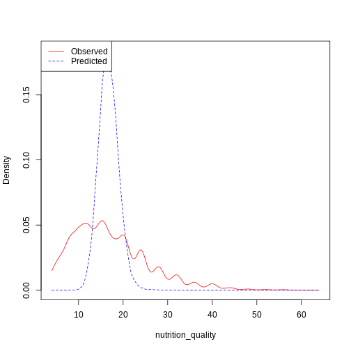
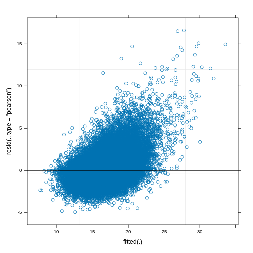
Validation
handover_boxplots(raw.dat, base.dat, v)
plot of chunk nutrition_validation
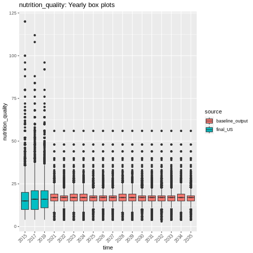
handover_lineplots(raw.dat, base.dat, v)
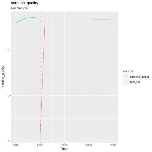
plot of chunk nutrition_validation
Results