Tobacco
Tobacco consumption is measured in the usual number of cigarettes smoked per day, and is taken directly from a US variable (ncigs). Number of cigarettes consumed is an indicator of several mental illnesses including anxiety (Lawrence et al. 2010).
continuous_density(obs)
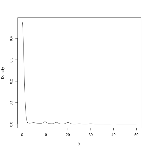
plot of chunk tobacco_data
obs_no_zero <- obs[obs != 0]  # remove zero values to look at counts only for smokers
continuous_density(obs_no_zero)
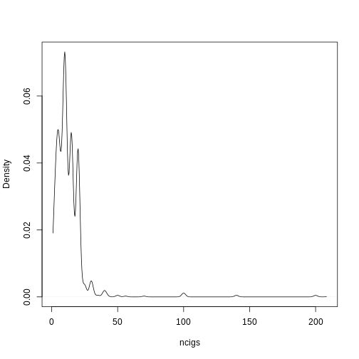
plot of chunk tobacco_data
Transition Model
The number of zero inflated values is higher than expected for a count
distribution such as a poisson distribution. This inflation occurs
naturally as a large proportion (over 50%) of the population do not
smoke. There are two sources of cigarette consumption that can be
modelled using zero inflated models. In this case a zero-inflated
poisson (ZIP) is used. Two models are fitted simultaneously. One is a
logistic regression that estimates whether a person smokes cigarettes or
not. This provides a simple probability of smoking or not. The second is
a poisson counts model estimating the number of cigarettes consumed.
This is modelled using the zeroinfl() function from the
pscl
package in R.
Formula:
NOTE: The syntax seen above I(ncigs>0) represents a binary flag for
whether a person smoked previously (ncigs > 0).
Two set of variables are needed for the logistic and poisson parts of the ZIP model respectively. These two formula are separated by a ‘|’ symbol. On the right hand side of the ‘|’ is the formula for the logistic regression that determines whether an individual is a smoker or not. On the left side is the formula for the poisson model to predict the counts of cigarettes for smokers.
Predictor |
Description |
Lite rature/Justification |
|---|---|---|
Previous Tobacco Consumption |
||
Sex |
||
Age |
||
Ethnicity |
||
Region |
Administrative region of the UK |
|
Education |
Highest attained qualification |
|
Household Income |
||
Behind on Bills |
||
Financial Situation |
zip_output(model)
##
## Call:
## zeroinfl(formula = formula, data = data, weights = weight, dist = "pois",
##     link = "logit")
##
## Pearson residuals:
##      Min       1Q   Median       3Q      Max
## -1.39165 -0.02575 -0.01822 -0.01256  7.88394
##
## Count model coefficients (poisson with log link):
##                                               Estimate Std. Error z value
## (Intercept)                                   1.756078   0.515096   3.409
## scale(age)                                    0.088226   0.072250   1.221
## factor(sex)Male                               0.132957   0.100926   1.317
## relevel(factor(ethnicity), ref = "WBI")BAN   -0.458047   0.724719  -0.632
## relevel(factor(ethnicity), ref = "WBI")BLA   -0.324150   0.524756  -0.618
## relevel(factor(ethnicity), ref = "WBI")BLC   -0.395408   0.500650  -0.790
## relevel(factor(ethnicity), ref = "WBI")CHI   -0.202406   1.083906  -0.187
## relevel(factor(ethnicity), ref = "WBI")IND   -0.222598   0.469511  -0.474
## relevel(factor(ethnicity), ref = "WBI")MIX   -0.343940   0.325918  -1.055
## relevel(factor(ethnicity), ref = "WBI")OAS   -0.604959   1.098497  -0.551
## relevel(factor(ethnicity), ref = "WBI")OBL   -0.423129   1.781472  -0.238
## relevel(factor(ethnicity), ref = "WBI")OTH    0.168325   0.534438   0.315
## relevel(factor(ethnicity), ref = "WBI")PAK   -0.852220   0.645376  -1.321
## relevel(factor(ethnicity), ref = "WBI")WHO    0.129127   0.178164   0.725
## factor(region)East of England                -0.207061   0.220486  -0.939
## factor(region)London                         -0.195256   0.224629  -0.869
## factor(region)North East                     -0.117416   0.263432  -0.446
## factor(region)North West                     -0.043274   0.201905  -0.214
## factor(region)Northern Ireland                0.013488   0.398038   0.034
## factor(region)Scotland                       -0.179701   0.257042  -0.699
## factor(region)South East                     -0.039395   0.207855  -0.190
## factor(region)South West                     -0.235811   0.227424  -1.037
## factor(region)Wales                          -0.045986   0.260487  -0.177
## factor(region)West Midlands                   0.122812   0.198825   0.618
## factor(region)Yorkshire and The Humber       -0.004834   0.211307  -0.023
## relevel(factor(education_state), ref = "1")0  0.422996   0.443084   0.955
## relevel(factor(education_state), ref = "1")2  0.362267   0.443040   0.818
## relevel(factor(education_state), ref = "1")3  0.157176   0.459963   0.342
## relevel(factor(education_state), ref = "1")5  0.199678   0.467004   0.428
## relevel(factor(education_state), ref = "1")6  0.103512   0.466882   0.222
## relevel(factor(education_state), ref = "1")7  0.497267   0.464812   1.070
## factor(housing_quality)Low                   -0.056672   0.175289  -0.323
## factor(housing_quality)Medium                -0.025581   0.117700  -0.217
## factor(loneliness)2                           0.164228   0.110798   1.482
## factor(loneliness)3                          -0.088262   0.187043  -0.472
## scale(nutrition_quality)                     -0.086828   0.057143  -1.519
## scale(ncigs)                                  0.060370   0.011383   5.303
## scale(hh_income)                             -0.047014   0.072999  -0.644
## scale(SF_12)                                 -0.042692   0.052335  -0.816
## factor(behind_on_bills)2                      0.032621   0.140519   0.232
## factor(behind_on_bills)3                     -0.223792   0.591207  -0.379
## factor(financial_situation)2                  0.132737   0.145536   0.912
## factor(financial_situation)3                  0.014451   0.167452   0.086
## factor(financial_situation)4                  0.047932   0.214865   0.223
## factor(financial_situation)5                 -0.059367   0.284620  -0.209
## factor(S7_labour_state)PT Employed           -0.012102   0.159718  -0.076
## factor(S7_labour_state)Job Seeking            0.137922   0.175851   0.784
## factor(S7_labour_state)FT Education          -0.389807   0.402215  -0.969
## factor(S7_labour_state)Family Care            0.172396   0.246076   0.701
## factor(S7_labour_state)Not Working            0.053776   0.146154   0.368
## factor(job_sec)1                              0.148942   0.307434   0.484
## factor(job_sec)2                             -0.006665   0.337203  -0.020
## factor(job_sec)3                              0.168864   0.214513   0.787
## factor(job_sec)4                              0.168856   0.225449   0.749
## factor(job_sec)5                              0.123171   0.230018   0.535
## factor(job_sec)6                              0.225291   0.225344   1.000
## factor(job_sec)7                              0.112134   0.208409   0.538
## factor(job_sec)8                              0.244970   0.226591   1.081
##                                              Pr(>|z|)
## (Intercept)                                  0.000651 ***
## scale(age)                                   0.222038
## factor(sex)Male                              0.187716
## relevel(factor(ethnicity), ref = "WBI")BAN   0.527365
## relevel(factor(ethnicity), ref = "WBI")BLA   0.536762
## relevel(factor(ethnicity), ref = "WBI")BLC   0.429651
## relevel(factor(ethnicity), ref = "WBI")CHI   0.851866
## relevel(factor(ethnicity), ref = "WBI")IND   0.635425
## relevel(factor(ethnicity), ref = "WBI")MIX   0.291290
## relevel(factor(ethnicity), ref = "WBI")OAS   0.581829
## relevel(factor(ethnicity), ref = "WBI")OBL   0.812256
## relevel(factor(ethnicity), ref = "WBI")OTH   0.752794
## relevel(factor(ethnicity), ref = "WBI")PAK   0.186668
## relevel(factor(ethnicity), ref = "WBI")WHO   0.468595
## factor(region)East of England                0.347674
## factor(region)London                         0.384715
## factor(region)North East                     0.655802
## factor(region)North West                     0.830289
## factor(region)Northern Ireland               0.972969
## factor(region)Scotland                       0.484482
## factor(region)South East                     0.849678
## factor(region)South West                     0.299792
## factor(region)Wales                          0.859872
## factor(region)West Midlands                  0.536781
## factor(region)Yorkshire and The Humber       0.981749
## relevel(factor(education_state), ref = "1")0 0.339748
## relevel(factor(education_state), ref = "1")2 0.413537
## relevel(factor(education_state), ref = "1")3 0.732565
## relevel(factor(education_state), ref = "1")5 0.668962
## relevel(factor(education_state), ref = "1")6 0.824541
## relevel(factor(education_state), ref = "1")7 0.284698
## factor(housing_quality)Low                   0.746463
## factor(housing_quality)Medium                0.827943
## factor(loneliness)2                          0.138279
## factor(loneliness)3                          0.637011
## scale(nutrition_quality)                     0.128639
## scale(ncigs)                                 1.14e-07 ***
## scale(hh_income)                             0.519552
## scale(SF_12)                                 0.414641
## factor(behind_on_bills)2                     0.816425
## factor(behind_on_bills)3                     0.705034
## factor(financial_situation)2                 0.361740
## factor(financial_situation)3                 0.931227
## factor(financial_situation)4                 0.823472
## factor(financial_situation)5                 0.834774
## factor(S7_labour_state)PT Employed           0.939602
## factor(S7_labour_state)Job Seeking           0.432859
## factor(S7_labour_state)FT Education          0.332469
## factor(S7_labour_state)Family Care           0.483564
## factor(S7_labour_state)Not Working           0.712916
## factor(job_sec)1                             0.628053
## factor(job_sec)2                             0.984231
## factor(job_sec)3                             0.431166
## factor(job_sec)4                             0.453871
## factor(job_sec)5                             0.592314
## factor(job_sec)6                             0.317424
## factor(job_sec)7                             0.590546
## factor(job_sec)8                             0.279648
##
## Zero-inflation model coefficients (binomial with logit link):
##                                            Estimate Std. Error z value Pr(>|z|)
## (Intercept)                                 5.32237    1.07790   4.938 7.90e-07
## I(factor(ncigs > 0))TRUE                   -4.69548    0.93360  -5.029 4.92e-07
## relevel(factor(ethnicity), ref = "WBI")BAN -0.50680    3.28346  -0.154    0.877
## relevel(factor(ethnicity), ref = "WBI")BLA -0.09712    2.29730  -0.042    0.966
## relevel(factor(ethnicity), ref = "WBI")BLC -1.14543    2.34089  -0.489    0.625
## relevel(factor(ethnicity), ref = "WBI")CHI -0.89546    3.71259  -0.241    0.809
## relevel(factor(ethnicity), ref = "WBI")IND  0.14328    2.26575   0.063    0.950
## relevel(factor(ethnicity), ref = "WBI")MIX -0.08254    2.00374  -0.041    0.967
## relevel(factor(ethnicity), ref = "WBI")OAS  0.39417    3.41132   0.116    0.908
## relevel(factor(ethnicity), ref = "WBI")OBL -0.43468    8.72959  -0.050    0.960
## relevel(factor(ethnicity), ref = "WBI")OTH  1.73849    3.39195   0.513    0.608
## relevel(factor(ethnicity), ref = "WBI")PAK  0.96084    2.13239   0.451    0.652
## relevel(factor(ethnicity), ref = "WBI")WHO -0.43313    1.21204  -0.357    0.721
## factor(housing_quality)Low                 -0.57763    1.15367  -0.501    0.617
## factor(housing_quality)Medium              -0.52553    0.70965  -0.741    0.459
## factor(loneliness)2                        -0.14139    0.74225  -0.190    0.849
## factor(loneliness)3                         0.13103    1.20400   0.109    0.913
## scale(nutrition_quality)                    0.05535    0.33362   0.166    0.868
## scale(ncigs)                               -0.62567    0.39396  -1.588    0.112
## relevel(factor(job_sec), ref = "3")0        0.05608    1.33826   0.042    0.967
## relevel(factor(job_sec), ref = "3")1       -0.80761    1.65422  -0.488    0.625
## relevel(factor(job_sec), ref = "3")2        0.02727    1.36350   0.020    0.984
## relevel(factor(job_sec), ref = "3")4       -0.33529    1.02164  -0.328    0.743
## relevel(factor(job_sec), ref = "3")5       -0.35811    1.21971  -0.294    0.769
## relevel(factor(job_sec), ref = "3")6       -0.49222    1.38210  -0.356    0.722
## relevel(factor(job_sec), ref = "3")7       -0.61393    0.94742  -0.648    0.517
## relevel(factor(job_sec), ref = "3")8       -0.68657    1.19747  -0.573    0.566
## scale(hh_income)                            0.05335    0.40103   0.133    0.894
## scale(SF_12)                                0.07009    0.34707   0.202    0.840
## factor(behind_on_bills)2                   -1.16405    1.15193  -1.011    0.312
## factor(behind_on_bills)3                    0.40170    5.17767   0.078    0.938
## factor(financial_situation)2               -0.12475    0.82111  -0.152    0.879
## factor(financial_situation)3               -0.52030    0.97033  -0.536    0.592
## factor(financial_situation)4               -0.17864    1.40060  -0.128    0.899
## factor(financial_situation)5               -1.09378    2.30711  -0.474    0.635
##
## (Intercept)                                ***
## I(factor(ncigs > 0))TRUE                   ***
## relevel(factor(ethnicity), ref = "WBI")BAN
## relevel(factor(ethnicity), ref = "WBI")BLA
## relevel(factor(ethnicity), ref = "WBI")BLC
## relevel(factor(ethnicity), ref = "WBI")CHI
## relevel(factor(ethnicity), ref = "WBI")IND
## relevel(factor(ethnicity), ref = "WBI")MIX
## relevel(factor(ethnicity), ref = "WBI")OAS
## relevel(factor(ethnicity), ref = "WBI")OBL
## relevel(factor(ethnicity), ref = "WBI")OTH
## relevel(factor(ethnicity), ref = "WBI")PAK
## relevel(factor(ethnicity), ref = "WBI")WHO
## factor(housing_quality)Low
## factor(housing_quality)Medium
## factor(loneliness)2
## factor(loneliness)3
## scale(nutrition_quality)
## scale(ncigs)
## relevel(factor(job_sec), ref = "3")0
## relevel(factor(job_sec), ref = "3")1
## relevel(factor(job_sec), ref = "3")2
## relevel(factor(job_sec), ref = "3")4
## relevel(factor(job_sec), ref = "3")5
## relevel(factor(job_sec), ref = "3")6
## relevel(factor(job_sec), ref = "3")7
## relevel(factor(job_sec), ref = "3")8
## scale(hh_income)
## scale(SF_12)
## factor(behind_on_bills)2
## factor(behind_on_bills)3
## factor(financial_situation)2
## factor(financial_situation)3
## factor(financial_situation)4
## factor(financial_situation)5
## ---
## Signif. codes:  0 '***' 0.001 '**' 0.01 '*' 0.05 '.' 0.1 ' ' 1
##
## Number of iterations in BFGS optimization: 62
## Log-likelihood: -225.5 on 93 Df
Validation
handover_boxplots(raw.dat, base.dat, v)
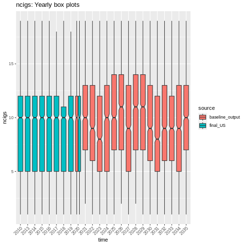
plot of chunk ncigs_validation
handover_lineplots(raw.dat, base.dat, v)
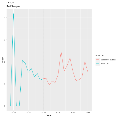
plot of chunk ncigs_validation
Results
Almost all coefficients significant. Particularly previous consumption of cigarettes. Good estimation of the number of non-smokers in the population at around 55%. Counts of smoking are underdispersed and fail to estimate consumption over 20 cigarettes.
## Error in density.default(obs, from = 0): argument 'x' must be numeric
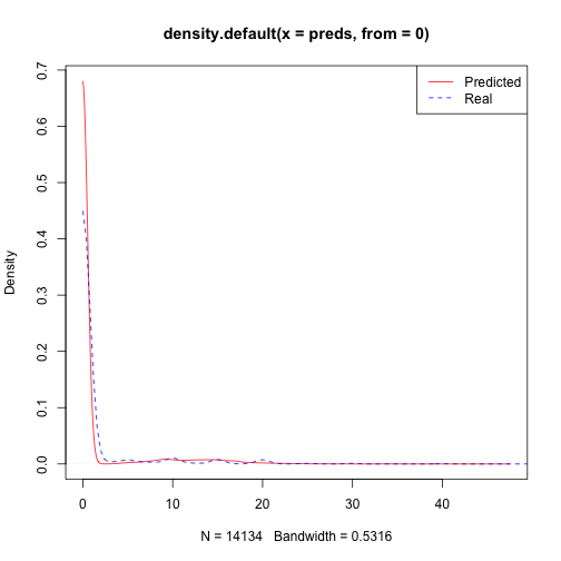
plot of chunk tobacco_output
References
Lawrence, David, Julie Considine, Francis Mitrou, and Stephen R Zubrick. 2010. “Anxiety Disorders and Cigarette Smoking: Results from the Australian Survey of Mental Health and Wellbeing.” Australian & New Zealand Journal of Psychiatry 44 (6): 520–27.