Labour
Labour state relates to the employment status of an individual, which is derived from the jbstat and jbft_dv variables from Understanding Society. The jbstat variable from US has 16 categories, which we have recoded into a variable with 6 categories based on the SIPHER 7 definition of labour state. jbft_dv indicates whether the individual worked full or part time (greater than 30 hours per week for full time). The table below shows which categories have been combined into the new reduced categories:
New Category |
Old Categories |
|---|---|
FT Employed |
Paid employment (AND jbft_dv == 1); Self-employed; Unpaid, family business; Apprenticeship; Furlough |
PT Employed |
Paid employment (AND jbft_dv == 2) |
Job Seeking |
Unemployed; Temporarily laid off/Short-term Working |
FT Education |
Full-time Student; Government Training |
Family Care |
Family Care |
Not Working |
Retired; Maternity Leave; LT Sick or Disabled |
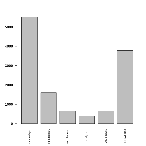
Fig. 21 plot of chunk labour_barchart
Transition Model
Labour state is a complex categorical data type. Single layer neural network is a simple way to estimate this state. Use multinom function from R’s nnet package. Formula for weights included given as.
Validation
handover_ordinal(raw.dat, base.dat, v)
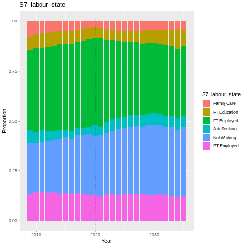
Fig. 22 plot of chunk S7_labour_state_validation
Results
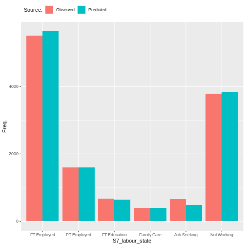
hard to determine goodness of fit.
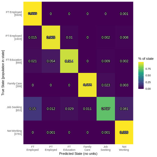
use confusion matrix to estimate quality of fit.
employed/retired well predicted. unemployed/student volatile socially and expectedly hard to predict.
some deterministic replacement needed for categories like student that have specific time frames. e.g. three years for a degree.
cumulative_link_plot(obs, preds)
## `geom_smooth()` using formula = 'y ~ x'
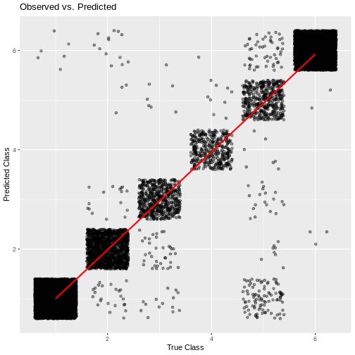
Fig. 23 plot of chunk labour_performance