Financial Situation

Financial Situation is a supplementary module in Minos. It is based on the finnow variable from Understanding Society, which represents an individuals current subjective financial situation. There are 5 levels of response; Living comfortably (1), Doing alright (2), Just about getting by (3), Finding it quite difficult (4), Finding it very difficult (5).

#discrete_barplot(obs, 'loneliness')
order <- c(1, 2, 3, 4, 5)
discrete_barplot(obs, order)

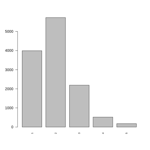
Fig. 50 plot of chunk fsitch_data

Transition Model

To predict the next state of financial_situation we use a Random Forest Ordinal model from the ranger package in R.

Formula:

\[\begin{split}financial\_situation \sim financial\_situation_last + age + sex + ethnicity + region\\ + education\_state + housing\_quality + neighbourhood\_safety\\ + loneliness + nutrition\_quality + ncigs + job\_sec\\ + hh\_income + marital\_status + housing\_tenure\end{split}\]

plot_rfo_importance(model)

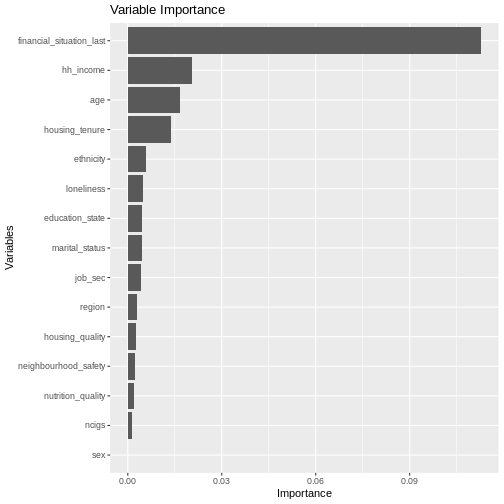
Fig. 51 plot of chunk fsitch_model_summary

Validation

handover_ordinal(raw.dat, base.dat, v)

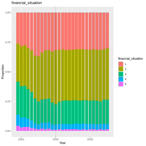
Fig. 52 plot of chunk fsitch_validation

pivoted <- combine_and_pivot_long(df1 = cv,
                                       df1.name = 'simulated',
                                       df2 = raw,
                                       df2.name = 'raw',
                                       var = v)

cv_ordinal_plots(pivoted.df = pivoted,
                 var = v,
                 save = FALSE)

## `summarise()` has grouped output by 'time', 'scenario'. You can override using
## the `.groups` argument.

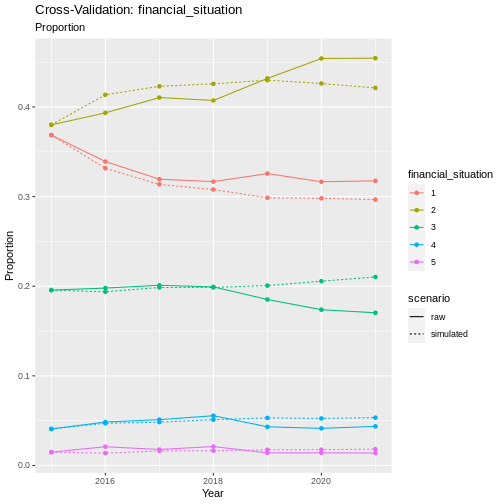
Fig. 53 plot of chunk fsitch_cv

Results

Random Forest Ordinal models from the ranger package cannot provide a summary like some other models can, so instead we will look at plots of observed vs predicted values as well as the importance of each variable in the resulting model.

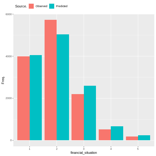
Fig. 54 plot of chunk fsitch_output

cumulative_link_plot(obs, preds)

## `geom_smooth()` using formula = 'y ~ x'

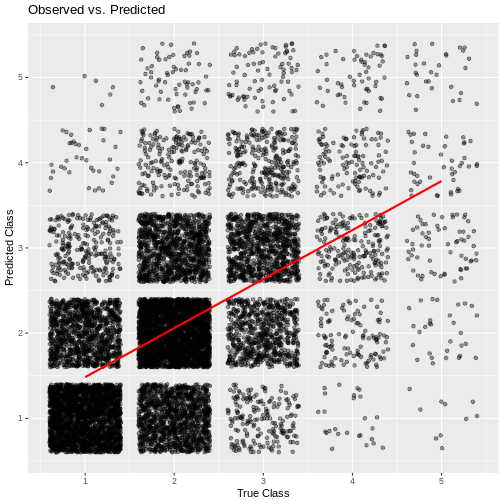
Fig. 55 plot of chunk fsitch_performance