Job NSSEC

Job NSSEC (known as job_sec in the model) refers to the eight category version of the National Statistics Socio-economic Classification (NS-SEC), and is taken directly from the jbnssec8_dv variable. See the table below for the categories and their value label:

Category	Value Label
Large employers and higher management	1
Higher professional	2
Lower management and professional	3
Intermediate	4
Small employers and own account	5
Lower supervisory and technical	6
Semi-routine	7
Routine	8
Not Employed	0

NOTE: Not Employed is a required category that is not part of the original variable (jbnssec8_dv). An unemployed person would have a missing value for job nssec and so has to be explicitly given one.

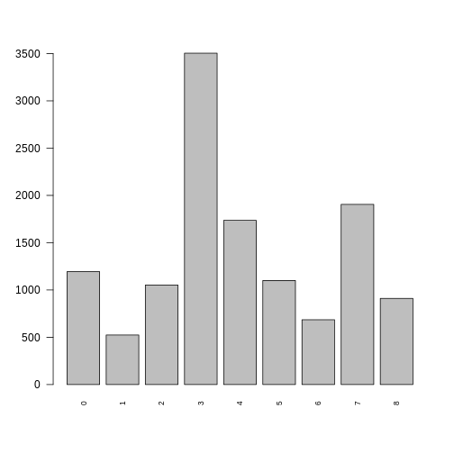
Fig. 56 plot of chunk job_sec_barchart

Transition Model

To predict the next state of job_sec we use a Random Forest Ordinal model from the ranger package in R.

Formula:

\[job\_sec \sim job\_sec\_last + age + sex + ethnicity + region + education\_state\]

plot_rfo_importance(model)

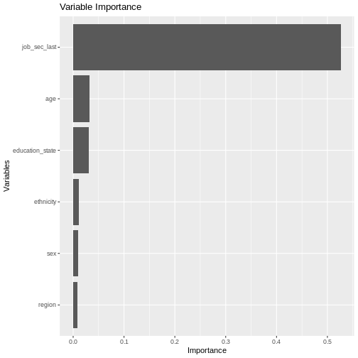
Fig. 57 plot of chunk job_sec_summary

Validation

handover_ordinal(raw.dat, base.dat, v)

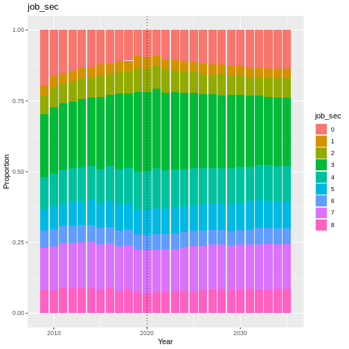
Fig. 58 plot of chunk bob_validation

pivoted <- combine_and_pivot_long(df1 = cv,
                                       df1.name = 'simulated',
                                       df2 = raw,
                                       df2.name = 'raw',
                                       var = v)

cv_ordinal_plots(pivoted.df = pivoted,
                 var = v,
                 save = FALSE)

## `summarise()` has grouped output by 'time', 'scenario'. You can override using
## the `.groups` argument.

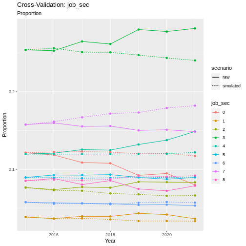
Fig. 59 plot of chunk bob_cv

Results

Random Forest Ordinal models from the ranger package cannot provide a summary like some other models can, so instead we will look at plots of observed vs predicted values as well as the importance of each variable in the resulting model.

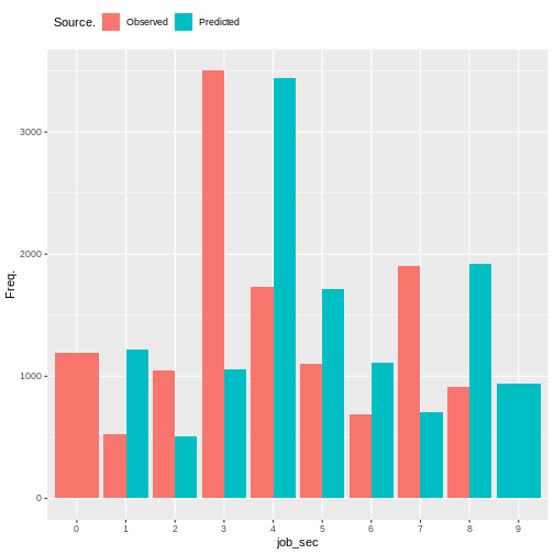
Fig. 60 plot of chunk bob_output

cumulative_link_plot(obs, preds)

## `geom_smooth()` using formula = 'y ~ x'

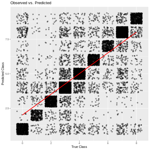
Fig. 61 plot of chunk bob_performance

References